
Next, we will analyze why the AND function wrongly returns FALSE:
- Hidden parameters of the function. As we will see below, it is very easy to make a mistake and introduce an extra empty parameter that causes the error. We will see two examples in which this case occurs and how to fix it.
- Values and formulas that return FALSE. You must be clear that the Excel AND function does not work wrongly, we are simply not able to realize what condition causes it to return a wrong value.
Except in the case of hidden parameters, the rest of the times where it returns FALSE is because one of its conditions is not TRUE and, as a consequence, the entire formula fails.
We will see two examples where we will realize that the Excel formula works correctly but we are not able to detect where it fails either because there are many values that are checked or we have many nested formulas.
Please note that if the IF function returns wrongly FALSE, it is because it uses the AND function or another similar function with identical problems and fixes, and therefore we will not focus on that function.
Hidden parameters of the AND function
The first reason why the Excel AND function returns wrongly FALSE is the “hidden parameters” that can be anywhere in it.
By hidden parameters I mean those that are in the Excel AND function without us realizing it because we have entered them by mistake. As an example of this we have the following:
=AND(TRUE;TRUE;)
=AND(TRUE;;TRUE)
If you look at the first function we have a hidden parameter at the end of it, and in the second function we have a hidden parameter in the middle. The previous examples are identical to the following:
=AND(TRUE;TRUE;FALSE)
=AND(TRUE;FALSE;TRUE)
Therefore, to fix the error of the Excel AND function returning wrongly FALSE, we must eliminate those additional parameters entered by mistake:
=AND(TRUE;TRUE)This is the only error that is not easy to detect at a glance, I spent an hour searching on the Internet until I realized that I had an extra semicolon at the end of the function.
Wrong values within the range cause FALSE return
This section, although it may also seem obvious, refers to checking the entire range in the Excel AND function, almost certainly one of the values is FALSE and you are not seeing it.
Let’s suppose we have the following case where we check a complete column of a table using the AND(D3:D8) function:

Although we don’t have an explicit FALSE in the values, we do have a 0 which is the same as FALSE and, as a consequence, the function that checks all the values will return FALSE.
Although it may seem easy to see in this example, if we had a range with 1000 records the matter would be a bit complicated, whether the value is FALSE or 0, it would be very difficult to find it.
Given the above, I recommend that you create an additional or supplementary column where you only check the value of the AND formula for the cell to its left, that is:
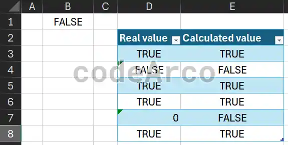
With this we will be able to clean the data and reduce it to only two possible values, FALSE and TRUE.
We would only have to filter the column we created to obtain only the “FALSE” values and thus see in which rows the general AND function is giving an error:

Simplify complex and nested formulas in AND
This last case is similar to the previous one and is based on the fact that we must avoid complex and nested formulas within AND in Excel to avoid possible confusion. When there are many nested functions with many levels, it is very difficult to find where the FALSE is.
Let’s look at the following example where, within the AND function, we have 3 EXACT formulas:

=AND(EXACT(D3;E3);EXACT(E3;F3);EXACT(F3;G3))The formula returns FALSE but… Why? Because the last condition is negative and, as a consequence, the entire formula is too.
My recommendation is that you separate these nested formulas into additional columns as shown in the following image:

And then within the AND function select the range of these additional columns:
=AND(H3:J3)With this you will be able to detect more precisely where the error is that makes the AND function not to be TRUE.
In fact, if you want to locate it much faster, you can create a conditional formatting rule in Excel through Home, Conditional Formatting, Manage Rules:

We establish the range to which the conditional formatting will be applied, in our case it is the row that contains the additional columns:
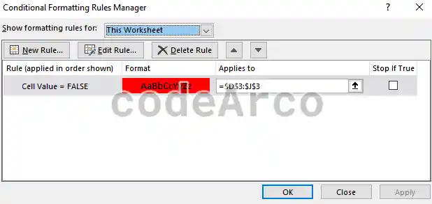
And finally select Edit rule, Format only cells that contain and, within it, select Cell value equal to “=FALSE”:

Finally we will be able to see the condition that causes our AND function to return FALSE more easily than if the function were nested:

As you have seen, the AND function in Excel never works badly or wrongly, it is always a human error, either because we have an extra parameter or because we are not able to detect where the condition is that causes the entire formula to fail.