Excel search for value in column and return another column

In this chapter we will see how to search for the value in column and return another in Excel through the following example:

• We have the following user data: ID, name and surname.
• We want to search for the user name in a column.
• Finally, we want to return the ID corresponding to the user that is in a different column, given the previous name.

We will also learn how to search in more complex scenarios where we do not only want to perform one search but several, one for each row of a table other than the one that contains the data.

Finally, we will see the power offered by Excel using wildcard characters to search in a more open and complex way, similar to regular expressions.

Simple example of searching in a column and returning a value

We will begin this tutorial with the necessary steps to search for a value in a column and return another:

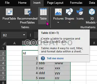
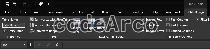
• Create a table with the data where we are going to perform the search. To do this, we go to “Insert, Table” with the previously selected data:
  

  

• Rename the table with a coherent name within “Table Design, Table Name”.
  In our case, we will use the name “TableData”, write it down for later, you will need it.
  

  

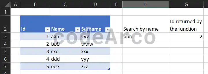
• Create two fields apart from the table to perform the search, one will be to enter the data we want to search for and the other will be where we will enter the Excel formula and it will return the corresponding value.
  In this case we are going to search by user name and we are going to return the corresponding id:
  

  

• We will enter, within the “Id returned” column, the following Excel formula:
  

  =INDICE(TableData[Id];COINCIDIR(F3;TableData[Name];0))

  =INDEX(TableData[Id];MATCH(F3;TableData[Name];0))

The explanation of the Excel formula is the following:

• The first parameter, TableData[Id], is the column that we will return if the search is successful.
• The second parameter, F3, will be the value to search for within the column.
• The third parameter, TableData[Name], is the column in which we will search for the value of the previous point.
• The fourth parameter, 0, indicates the type of match. In our case we will use 0 to indicate that we want exact matches. If you need more information about this parameter, you can check it on the official Microsoft page about the match formula.

Finally, you can play around by changing the name and you will see that it returns the corresponding id or “#N/D” in case it does not find an exact match.

Wildcard characters to search in Excel

If we want to enhance the previous search, we can use Excel’s wildcard characters both in the value to search for and in the formula we have used. Some examples of Excel wildcard characters are:

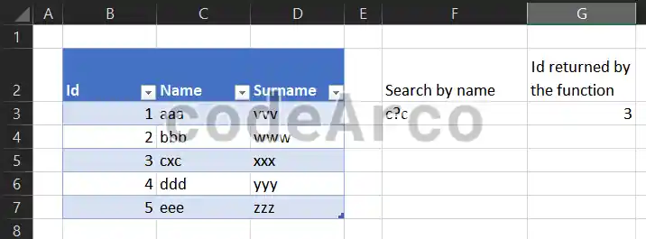
• Using the question mark “?” in the search value, if we enter “c?c” we will be searching for the user ID whose name has a “c” followed by any character and followed by another “c”:
  

  

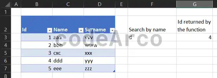
• Using the asterisk “*” in the formula we can tell Excel to search for the user whose first letter of the name begins with what we enter in the search cell:
  

  =INDICE(TableData[Id];COINCIDIR(F3&"*";TableData[Name];0))

  =INDEX(TableData[Id];MATCH(F3&"*";TableData[Name];0))

  

Advanced example to search and return values ​​in Excel

There are more complex scenarios where, for example, we want to search for each row of a table for a cell in another table and, if it is found, return a specific cell from that other table.

The solution is simple, you just have to use the formula above for each row of the new table mentioning the table where we will search, that is:

=INDICE(TableData[Id];COINCIDIR([NameToSearch];TableData[Name];0))

=INDEX(TableData[Id];MATCH([NameToSearch];TableData[Name];0))

The only thing that changes is that the value to search for, before it was F3, now it is not a single value but an entire column and, therefore, we must change it to the name of the specific column which in this case is [NameToSearch].