VLOOKUP not working, fix #N/A error in Excel

The VLOOKUP function allows you to look up a value in a column of an Excel table and return the corresponding value from another column.

Although it is very useful, the truth is that it generates many headaches because it often does not work as expected.

That is why below we will see some of the possible errors and how to fix the #N/A error for VLOOKUP.

VLOOKUP example working and fixed

Let’s start by using the following VLOOKUP example that works correctly. In it we have created a table with the data we have through the “Insert, Table” menu after selecting the data range and, subsequently, we have given it a name through the “Table Design, Table Name” menu:

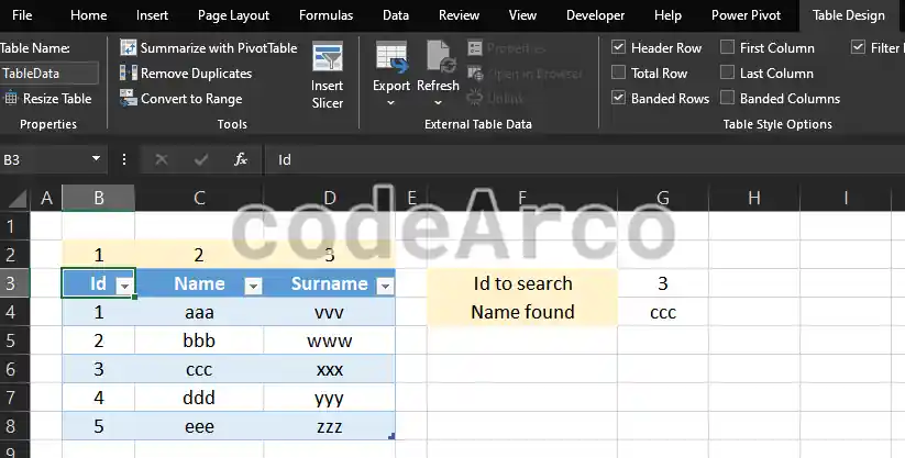
We have also created two additional cells:

Id to search, will be the value that we will search for in the table to return its corresponding name.
Name found, this is where we will use the VLOOKUP function with the following values:
```
=VLOOKUP(G3;TableData;2)
```

As you can see, it is working correctly and the parameters of the VLOOKUP function are:

First parameter, indicates the value to search for, in this case it is cell G3 which corresponds to the id we will insert.
Second parameter, indicates where we will search. It can be a range such as, for example, “B5:D8”, or we can use a reference to a full table through its name as in the example where we used “TableData”.
Third parameter, indicates the column within the previous range to return. The columns are numbered starting with 1, from left to right. In this case, since we want to return the name, we will use the value 2.

You can play with the example and change values, perform searches… etc to check that it is working correctly.

Incorrect range returns error #N/A

The first most common mistake is not understanding how Excel’s VLOOKUP function works. This function searches only in the first column of the search range, that is, the one on the far left.

Let’s suppose that in our example we want to search by name and return the last name. Well, if we don’t modify the formula we will see that we get the famous #N/A error:

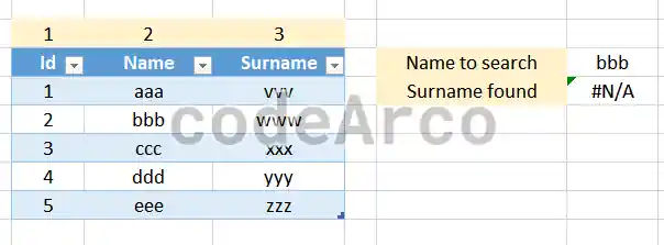
In this case the fix for the #N/A error is simple, we simply have to modify the range in which the search is performed, that is, the second parameter of the VLOOKUP formula.

The formula before the modification was:

=VLOOKUP(G3;TableData;2)

And the modified formula to fix the #N/A error is:

=VLOOKUP(G3;TableData[[Name]:[Surname]];2)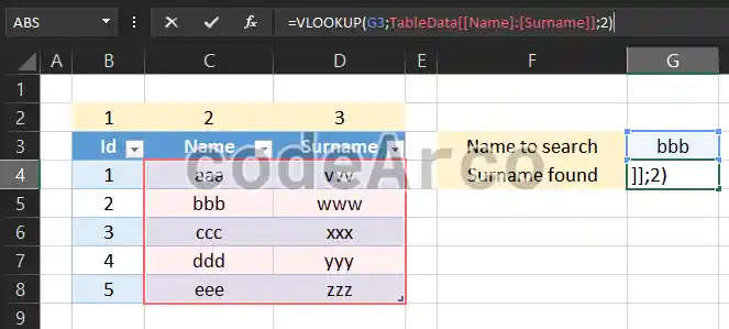

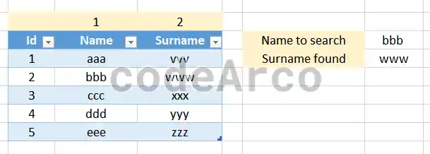
With this modification we will get the formula to search in the first column of the range that is now the first name and find it, thus returning the corresponding last name:

Use exact matches in VLOOKUP

You may have noticed that if we search for the name “dd” it returns the surname “xxx” and this is incorrect because the name “dd” does not exist:

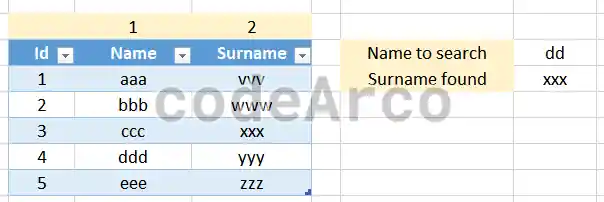
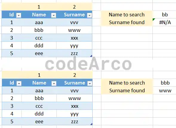
Well, my recommendation is that you add a fourth parameter to the previous formula with the value FALSE so that it only searches for exact matches and not approximate matches:

=VLOOKUP(G3;TableData[[Name]:[Surname]];2;FALSE)

With this we will ensure that if the match is not exact it will throw the famous #N/A error and in this way we will avoid possible misunderstandings:

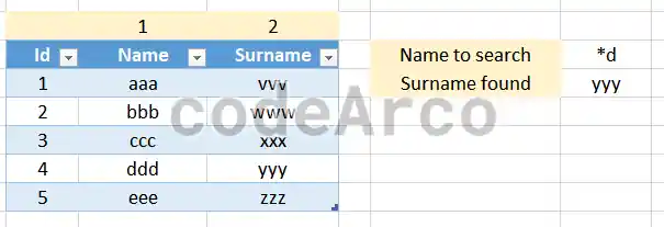
Now, what happens if I want more advanced functionality similar to regular expressions? My recommendation is to use exact matches in combination with Excel wildcards. In the following example we will search for a name that ends with the letter “d” and it will return the corresponding last name:

N/A error due to incorrect column order

Let’s think for a moment about what it means that the VLOOKUP formula searches in the first column of the selected range… This means that:

The column where we will search must necessarily be the first column of the range used in the formula.
The column from which we will return the value must necessarily be to the right of the column where we search (not immediately after, there may be columns in between).

This has the following problem… What happens if we want to search in a column that is to the right of the return column? Following our example, what happens if we want to search by last name and return the corresponding id?

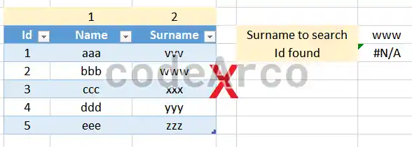
Well, in the previous scenario the VLOOKUP function does not work, we cannot use it directly. We can fix this type of error with:

Change the order of the columns so that, at least, the column in which we search is to the left of the column from which we will return the value.
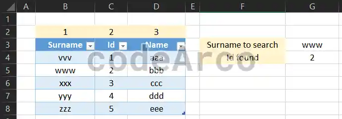
Following our example, we must to move the “Surname” column to the left of the “Id” column and use the formula as we did in previous sections:
Fix error with incorrect column order
```
=VLOOKUP(G3;TableData;2)
```
Use a better alternative to the VLOOKUP function that allows us to explicitly indicate which column we will search and which column we will return.
In the linked post you have all the instructions to search for a column and return another without the problems generated by the VLOOKUP formula.
This is the recommended option for searching for one column and returning another. It is the cleanest and most powerful way. Personally, I prefer not to have to change the order of columns in complex files because of the consequences that this may have.
Another advantage of the fix described is that we are not forced to have the columns in a certain order for the searches to be successful, they can be in any order and they will always work.

Incorrect data format in VLOOKUP

Another very common error when using VLOOKUP is that the data we are looking for does not have the same format as the column where we are looking.

In the following example we can see that we are looking in a column with a number format and that the value searched is in text format. As a consequence we will get, again, the error #N/A:

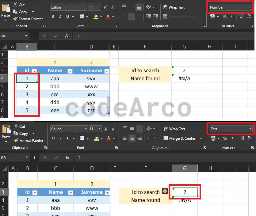
Here the fix is simple, just put both with the same format, or both in text format or both in number format.

Blank spaces generate the error #N/A

Finally we will see another error in the VLOOKUP function that is not so frequent but that also generates the error #N/A. This error is due to blank spaces, either in the searched value or in the lookup column:

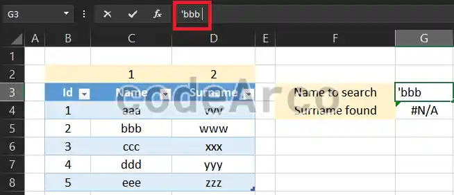
To fix this error, use the TRIM formula within the first parameter of VLOOKUP:

=VLOOKUP(TRIM(G3);TableData[[Name]:[Surname]];2;FALSE)

If the error persists, it is because the space is in the lookup column. The only fix here is to manually modify the data and remove those extra spaces, although you can also create a second column to clean up the blank spaces with the previous function.